01-pandas-titanic

1. 数据分析实际案例之：pandas在泰坦尼特号乘客数据中的使用

简介

1912年4月15日，号称永不沉没的泰坦尼克号因为和冰山相撞沉没了。因为没有足够的救援设备，2224个乘客中有1502个乘客不幸遇难。事故已经发生了，但是我们可以从泰坦尼克号中的历史数据中发现一些数据规律吗？今天本文将会带领大家灵活的使用pandas来进行数据分析。

泰坦尼特号乘客数据

我们从kaggle官网中下载了部分泰坦尼特号的乘客数据，主要包含下面几个字段：

变量名	含义	取值
survival	是否生还	0 = No, 1 = Yes
pclass	船票的级别	1 = 1st, 2 = 2nd, 3 = 3rd
sex	性别
Age	年龄
sibsp	配偶信息
parch	父母或者子女信息
ticket	船票编码
fare	船费
cabin	客舱编号
embarked	登录的港口	C = Cherbourg, Q = Queenstown, S = Southampton

下载下来的文件是一个csv文件。接下来我们来看一下怎么使用pandas来对其进行数据分析。

使用pandas对数据进行分析

引入依赖包

本文主要使用pandas和matplotlib，所以需要首先进行下面的通用设置：

from numpy.random import randn
import numpy as np
np.random.seed(123)
import os
import matplotlib.pyplot as plt
import pandas as pd
plt.rc('figure', figsize=(10, 6))
np.set_printoptions(precision=4)
pd.options.display.max_rows = 20

读取和分析数据

pandas提供了一个read_csv方法可以很方便的读取一个csv数据，并将其转换为DataFrame：

path = '../data/titanic.csv'
df = pd.read_csv(path)
df

我们看下读入的数据：

PassengerId	Pclass	Name	Sex	Age	SibSp	Parch	Ticket	Fare	Cabin	Embarked
0	892	3	Kelly, Mr. James	male	34.5	0	0	330911	7.8292	NaN	Q
1	893	3	Wilkes, Mrs. James (Ellen Needs)	female	47.0	1	0	363272	7.0000	NaN	S
2	894	2	Myles, Mr. Thomas Francis	male	62.0	0	0	240276	9.6875	NaN	Q
3	895	3	Wirz, Mr. Albert	male	27.0	0	0	315154	8.6625	NaN	S
4	896	3	Hirvonen, Mrs. Alexander (Helga E Lindqvist)	female	22.0	1	1	3101298	12.2875	NaN	S
5	897	3	Svensson, Mr. Johan Cervin	male	14.0	0	0	7538	9.2250	NaN	S
6	898	3	Connolly, Miss. Kate	female	30.0	0	0	330972	7.6292	NaN	Q
7	899	2	Caldwell, Mr. Albert Francis	male	26.0	1	1	248738	29.0000	NaN	S
8	900	3	Abrahim, Mrs. Joseph (Sophie Halaut Easu)	female	18.0	0	0	2657	7.2292	NaN	C
9	901	3	Davies, Mr. John Samuel	male	21.0	2	0	A/4 48871	24.1500	NaN	S
...	...	...	...	...	...	...	...	...	...	...	...
408	1300	3	Riordan, Miss. Johanna Hannah""	female	NaN	0	0	334915	7.7208	NaN	Q
409	1301	3	Peacock, Miss. Treasteall	female	3.0	1	1	SOTON/O.Q. 3101315	13.7750	NaN	S
410	1302	3	Naughton, Miss. Hannah	female	NaN	0	0	365237	7.7500	NaN	Q
411	1303	1	Minahan, Mrs. William Edward (Lillian E Thorpe)	female	37.0	1	0	19928	90.0000	C78	Q
412	1304	3	Henriksson, Miss. Jenny Lovisa	female	28.0	0	0	347086	7.7750	NaN	S
413	1305	3	Spector, Mr. Woolf	male	NaN	0	0	A.5. 3236	8.0500	NaN	S
414	1306	1	Oliva y Ocana, Dona. Fermina	female	39.0	0	0	PC 17758	108.9000	C105	C
415	1307	3	Saether, Mr. Simon Sivertsen	male	38.5	0	0	SOTON/O.Q. 3101262	7.2500	NaN	S
416	1308	3	Ware, Mr. Frederick	male	NaN	0	0	359309	8.0500	NaN	S
417	1309	3	Peter, Master. Michael J	male	NaN	1	1	2668	22.3583	NaN	C

418 rows × 11 columns

调用df的describe方法可以查看基本的统计信息：

	PassengerId	Pclass	Age	SibSp	Parch	Fare
count	418.000000	418.000000	332.000000	418.000000	418.000000	417.000000
mean	1100.500000	2.265550	30.272590	0.447368	0.392344	35.627188
std	120.810458	0.841838	14.181209	0.896760	0.981429	55.907576
min	892.000000	1.000000	0.170000	0.000000	0.000000	0.000000
25%	996.250000	1.000000	21.000000	0.000000	0.000000	7.895800
50%	1100.500000	3.000000	27.000000	0.000000	0.000000	14.454200
75%	1204.750000	3.000000	39.000000	1.000000	0.000000	31.500000
max	1309.000000	3.000000	76.000000	8.000000	9.000000	512.329200

如果要想查看乘客登录的港口，可以这样选择：

df['Embarked'][:10]

0    Q
1    S
2    Q
3    S
4    S
5    S
6    Q
7    S
8    C
9    S
Name: Embarked, dtype: object

使用value_counts 可以对其进行统计：

embark_counts=df['Embarked'].value_counts()
embark_counts[:10]

S    270
C    102
Q     46
Name: Embarked, dtype: int64

从结果可以看出，从S港口登录的乘客有270个，从C港口登录的乘客有102个，从Q港口登录的乘客有46个。

同样的，我们可以统计一下age信息：

age_counts=df['Age'].value_counts()
age_counts.head(10)

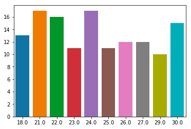
前10位的年龄如下：

24.0    17
21.0    17
22.0    16
30.0    15
18.0    13
27.0    12
26.0    12
25.0    11
23.0    11
29.0    10
Name: Age, dtype: int64

计算一下年龄的平均数：

df['Age'].mean()

30.272590361445783

实际上有些数据是没有年龄的，我们可以使用平均数对其填充：

clean_age1 = df['Age'].fillna(df['Age'].mean())
clean_age1.value_counts()

可以看出平均数是30.27，个数是86。

30.27259    86
24.00000    17
21.00000    17
22.00000    16
30.00000    15
18.00000    13
26.00000    12
27.00000    12
25.00000    11
23.00000    11
            ..
36.50000     1
40.50000     1
11.50000     1
34.00000     1
15.00000     1
7.00000      1
60.50000     1
26.50000     1
76.00000     1
34.50000     1
Name: Age, Length: 80, dtype: int64

使用平均数来作为年龄可能不是一个好主意，还有一种办法就是丢弃平均数：

clean_age2=df['Age'].dropna()
clean_age2
age_counts = clean_age2.value_counts()
ageset=age_counts.head(10)
ageset

24.0    17
21.0    17
22.0    16
30.0    15
18.0    13
27.0    12
26.0    12
25.0    11
23.0    11
29.0    10
Name: Age, dtype: int64

图形化表示和矩阵转换

图形化对于数据分析非常有帮助，我们对于上面得出的前10名的age使用柱状图来表示：

import seaborn as sns
sns.barplot(x=ageset.index, y=ageset.values)

接下来我们来做一个复杂的矩阵变换，我们先来过滤掉age和sex都为空的数据：

cframe=df[df.Age.notnull() & df.Sex.notnull()]
cframe

	PassengerId	Pclass	Name	Sex	Age	SibSp	Parch	Ticket	Fare	Cabin	Embarked
0	892	3	Kelly, Mr. James	male	34.5	0	0	330911	7.8292	NaN	Q
1	893	3	Wilkes, Mrs. James (Ellen Needs)	female	47.0	1	0	363272	7.0000	NaN	S
2	894	2	Myles, Mr. Thomas Francis	male	62.0	0	0	240276	9.6875	NaN	Q
3	895	3	Wirz, Mr. Albert	male	27.0	0	0	315154	8.6625	NaN	S
4	896	3	Hirvonen, Mrs. Alexander (Helga E Lindqvist)	female	22.0	1	1	3101298	12.2875	NaN	S
5	897	3	Svensson, Mr. Johan Cervin	male	14.0	0	0	7538	9.2250	NaN	S
6	898	3	Connolly, Miss. Kate	female	30.0	0	0	330972	7.6292	NaN	Q
7	899	2	Caldwell, Mr. Albert Francis	male	26.0	1	1	248738	29.0000	NaN	S
8	900	3	Abrahim, Mrs. Joseph (Sophie Halaut Easu)	female	18.0	0	0	2657	7.2292	NaN	C
9	901	3	Davies, Mr. John Samuel	male	21.0	2	0	A/4 48871	24.1500	NaN	S
...	...	...	...	...	...	...	...	...	...	...	...
403	1295	1	Carrau, Mr. Jose Pedro	male	17.0	0	0	113059	47.1000	NaN	S
404	1296	1	Frauenthal, Mr. Isaac Gerald	male	43.0	1	0	17765	27.7208	D40	C
405	1297	2	Nourney, Mr. Alfred (Baron von Drachstedt")"	male	20.0	0	0	SC/PARIS 2166	13.8625	D38	C
406	1298	2	Ware, Mr. William Jeffery	male	23.0	1	0	28666	10.5000	NaN	S
407	1299	1	Widener, Mr. George Dunton	male	50.0	1	1	113503	211.5000	C80	C
409	1301	3	Peacock, Miss. Treasteall	female	3.0	1	1	SOTON/O.Q. 3101315	13.7750	NaN	S
411	1303	1	Minahan, Mrs. William Edward (Lillian E Thorpe)	female	37.0	1	0	19928	90.0000	C78	Q
412	1304	3	Henriksson, Miss. Jenny Lovisa	female	28.0	0	0	347086	7.7750	NaN	S
414	1306	1	Oliva y Ocana, Dona. Fermina	female	39.0	0	0	PC 17758	108.9000	C105	C
415	1307	3	Saether, Mr. Simon Sivertsen	male	38.5	0	0	SOTON/O.Q. 3101262	7.2500	NaN	S

332 rows × 11 columns

接下来使用groupby对age和sex进行分组：

by_sex_age = cframe.groupby(['Age', 'Sex'])
by_sex_age.size()

Age    Sex   
0.17   female    1
0.33   male      1
0.75   male      1
0.83   male      1
0.92   female    1
1.00   female    3
2.00   female    1
       male      1
3.00   female    1
5.00   male      1
                ..
60.00  female    3
60.50  male      1
61.00  male      2
62.00  male      1
63.00  female    1
       male      1
64.00  female    2
       male      1
67.00  male      1
76.00  female    1
Length: 115, dtype: int64

使用unstack将Sex的列数据变成行：

Sex	female	male
Age
0.17	1.0	0.0
0.33	0.0	1.0
0.75	0.0	1.0
0.83	0.0	1.0
0.92	1.0	0.0
1.00	3.0	0.0
2.00	1.0	1.0
3.00	1.0	0.0
5.00	0.0	1.0
6.00	0.0	3.0
...	...	...
58.00	1.0	0.0
59.00	1.0	0.0
60.00	3.0	0.0
60.50	0.0	1.0
61.00	0.0	2.0
62.00	0.0	1.0
63.00	1.0	1.0
64.00	2.0	1.0
67.00	0.0	1.0
76.00	1.0	0.0

79 rows × 2 columns

我们把同样age的人数加起来，然后使用argsort进行排序，得到排序过后的index：

indexer = agg_counts.sum(1).argsort()
indexer.tail(10)

Age
58.0    37
59.0    31
60.0    29
60.5    32
61.0    34
62.0    22
63.0    38
64.0    27
67.0    26
76.0    30
dtype: int64

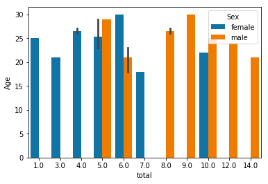
从agg_counts中取出最后的10个，也就是最大的10个：

count_subset = agg_counts.take(indexer.tail(10))
count_subset=count_subset.tail(10)
count_subset

Sex	female	male
Age
29.0	5.0	5.0
25.0	1.0	10.0
23.0	5.0	6.0
26.0	4.0	8.0
27.0	4.0	8.0
18.0	7.0	6.0
30.0	6.0	9.0
22.0	10.0	6.0
21.0	3.0	14.0
24.0	5.0	12.0

上面的操作可以简化为下面的代码：

agg_counts.sum(1).nlargest(10)

Age
21.0    17.0
24.0    17.0
22.0    16.0
30.0    15.0
18.0    13.0
26.0    12.0
27.0    12.0
23.0    11.0
25.0    11.0
29.0    10.0
dtype: float64

将count_subset 进行stack操作，方便后面的画图：

stack_subset = count_subset.stack()
stack_subset

Age   Sex   
29.0  female     5.0
      male       5.0
25.0  female     1.0
      male      10.0
23.0  female     5.0
      male       6.0
26.0  female     4.0
      male       8.0
27.0  female     4.0
      male       8.0
18.0  female     7.0
      male       6.0
30.0  female     6.0
      male       9.0
22.0  female    10.0
      male       6.0
21.0  female     3.0
      male      14.0
24.0  female     5.0
      male      12.0
dtype: float64

stack_subset.name = 'total'
stack_subset = stack_subset.reset_index()
stack_subset

Age	Sex	total
0	29.0	female	5.0
1	29.0	male	5.0
2	25.0	female	1.0
3	25.0	male	10.0
4	23.0	female	5.0
5	23.0	male	6.0
6	26.0	female	4.0
7	26.0	male	8.0
8	27.0	female	4.0
9	27.0	male	8.0
10	18.0	female	7.0
11	18.0	male	6.0
12	30.0	female	6.0
13	30.0	male	9.0
14	22.0	female	10.0
15	22.0	male	6.0
16	21.0	female	3.0
17	21.0	male	14.0
18	24.0	female	5.0
19	24.0	male	12.0

作图如下：

sns.barplot(x='total', y='Age', hue='Sex',  data=stack_subset)

本文例子可以参考： https://github.com/ddean2009/learn-ai/